
Installation
# Install from CRAN
install.packages("ggadjustedforest")

# Or install the development version from GitHub
# install.packages("remotes")
remotes::install_github("kriz98/ggadjustedforest")
Motivation
When building multivariable models for causal inference, there is an exposure of interest for which a causal estimand applies to. The coefficients for adjusted covariates (confounders) can however be misinterpreted when presented together with the effect estimate of interest. Reporting them can even mislead readers, because confounder coefficients are not identified under the causal model, and are susceptible to absorbing collider bias, mediation pathways, and other artefacts depending on causal structures (Hernán & Robins, Causal Inference: What If, 2020; Westreich & Greenland, Am J Epidemiol, 2013).
STROBE guidelines (Vandenbroucke et al., 2007) and recent work on the estimand framework (ICH E9(R1), 2019) both emphasise that reporting should clearly distinguish the target quantity from nuisance parameters.
ggadjustedforest operationalises these principles and
fits the models you specify but only exposes the effect of
interest in both the forest plots and associated tables, hiding
confounder estimates by design.
An additional feature for exploratory data analysis is also provided whereby the cumulative addition of covariates can be investigated.
Data
All examples use the rotterdam breast cancer dataset
from the survival package — 2,982 primary breast cancer
patients from the Rotterdam tumour bank. The research question
throughout is whether hormonal therapy (hormon) affects
survival and recurrence, before and after adjusting for patient and
tumour characteristics.
library(ggadjustedforest)
#> ggadjustedforest 0.1.1 -- Forest plots for exposure effects, hiding confounders by design.
#> See `?gg_adjusted_forest` to get started.
library(dplyr)
#>
#> Attaching package: 'dplyr'
#> The following objects are masked from 'package:stats':
#>
#>     filter, lag
#> The following objects are masked from 'package:base':
#>
#>     intersect, setdiff, setequal, union
data(cancer, package = "survival")

df <- rotterdam |>
  transmute(
    hormon = hormon,   # 1 = hormonal therapy, 0 = none
    age    = age,
    size   = size,     # tumour size (mm)
    grade  = grade,    # tumour grade
    nodes  = nodes,    # positive lymph nodes
    er10   = er / 10,  # oestrogen receptor (fmol/10 l)
    recur  = recur,    # recurrence (0/1)
    death  = death,    # all-cause death (0/1)
    rtime  = rtime,    # time to recurrence/censoring
    dtime  = dtime     # time to death/censoring
  ) |>
  tidyr::drop_na()

covariates <- c("age", "size", "grade", "nodes", "er10")
Basic usage — logistic regression
The pipe-friendly API puts data first so the function
composes naturally with |>:
result <- df |>
  gg_adjusted_forest(
    outcome    = "death",
    exposure   = "hormon",
    covariates = covariates,
    model_type = "logistic",
    title      = "Effect of Hormonal Therapy on Death (Logistic)"
  )
result$table
#> # A tibble: 2 × 6
#>   model      estimate conf.low conf.high     p.value     n
#>   <fct>         <dbl>    <dbl>     <dbl>       <dbl> <int>
#> 1 Unadjusted    1.21     0.967     1.52  0.0935       2982
#> 2 Adjusted      0.499    0.381     0.652 0.000000411  2982
The returned object has three components:
| Component | Contents |
|---|---|
$plot |
Combined forest plot + table (ggplot2 / patchwork) |
$table |
Tibble of numeric estimates |
$formatted_table |
Tibble with formatted “OR (lower–upper)” strings |
To render the plot:
result$plot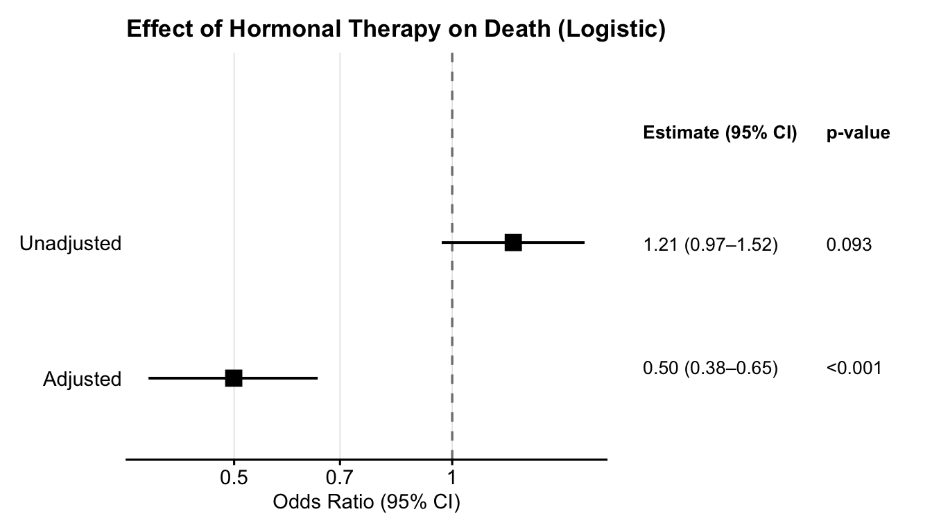
Cumulative adjustment
Although generally recommended against when performing causal inference, sequential addition of covariates may be helpful when building regression models for predictive and descriptive aims. As such, this feature is provided to visualise how the effect estimate changes as covariates are added sequentially. This may aid in the selection of a parsimonious model with the best fit as recommended by the principles laid out in R for Health Data Science by Ewen Harrison and Riinu Pius.
Collapsibility and interpreting sequential estimates
A key consideration when using cumulative adjustment is whether the effect measure being modelled is collapsible. A collapsible effect measure is one where the marginal (unadjusted) estimate equals a weighted average of the stratum-specific (adjusted) estimates. For collapsible measures, a change in the exposure coefficient as covariates are added can be interpreted as evidence of confounding. For non-collapsible measures, the coefficient changes simply because adding covariates alters the residual variance on the underlying latent scale, even when there is no confounding at all.
| Model type | Effect measure | Collapsible | Cumulative display interpretable? |
|---|---|---|---|
"linear" |
Risk difference | ✅ Yes | ✅ Yes |
"poisson" |
Risk ratio | ✅ Yes | ✅ Yes |
"logistic" |
Odds ratio | ❌ No | ⚠️ Use with caution |
"coxph" |
Hazard ratio | ❌ No | ⚠️ Use with caution |
When cumulative = TRUE is used with
"logistic" or "coxph",
ggadjustedforest will emit a warning to this effect. The
feature is retained because it remains useful in descriptive and
predictive modelling contexts — for example, when assessing whether
model fit improves with each additional covariate, but the sequential
change in OR or HR should not be interpreted as a direct measure of
confounding.
For a full treatment of non-collapsibility see Greenland (1987) and Hernán (2010).
To use this feature, set cumulative = TRUE and use
cumulative_labels to provide human-readable row names:
result_cum <- gg_adjusted_forest(
  data       = df,
  outcome    = "death",
  exposure   = "hormon",
  covariates = covariates,
  model_type = "logistic",
  cumulative = TRUE,
  cumulative_labels = c(
    "Unadjusted"                       = "Unadjusted",
    "+ age"                            = "+ Age",
    "+ age + size"                     = "+ Tumour size",
    "+ age + size + grade"             = "+ Grade",
    "+ age + size + grade + nodes"     = "+ Lymph nodes",
    "+ age + size + grade + nodes + er10" = "+ Oestrogen receptor"
  ),
  title = "Cumulative Adjustment: Hormonal Therapy on Death"
)
result_cum$plot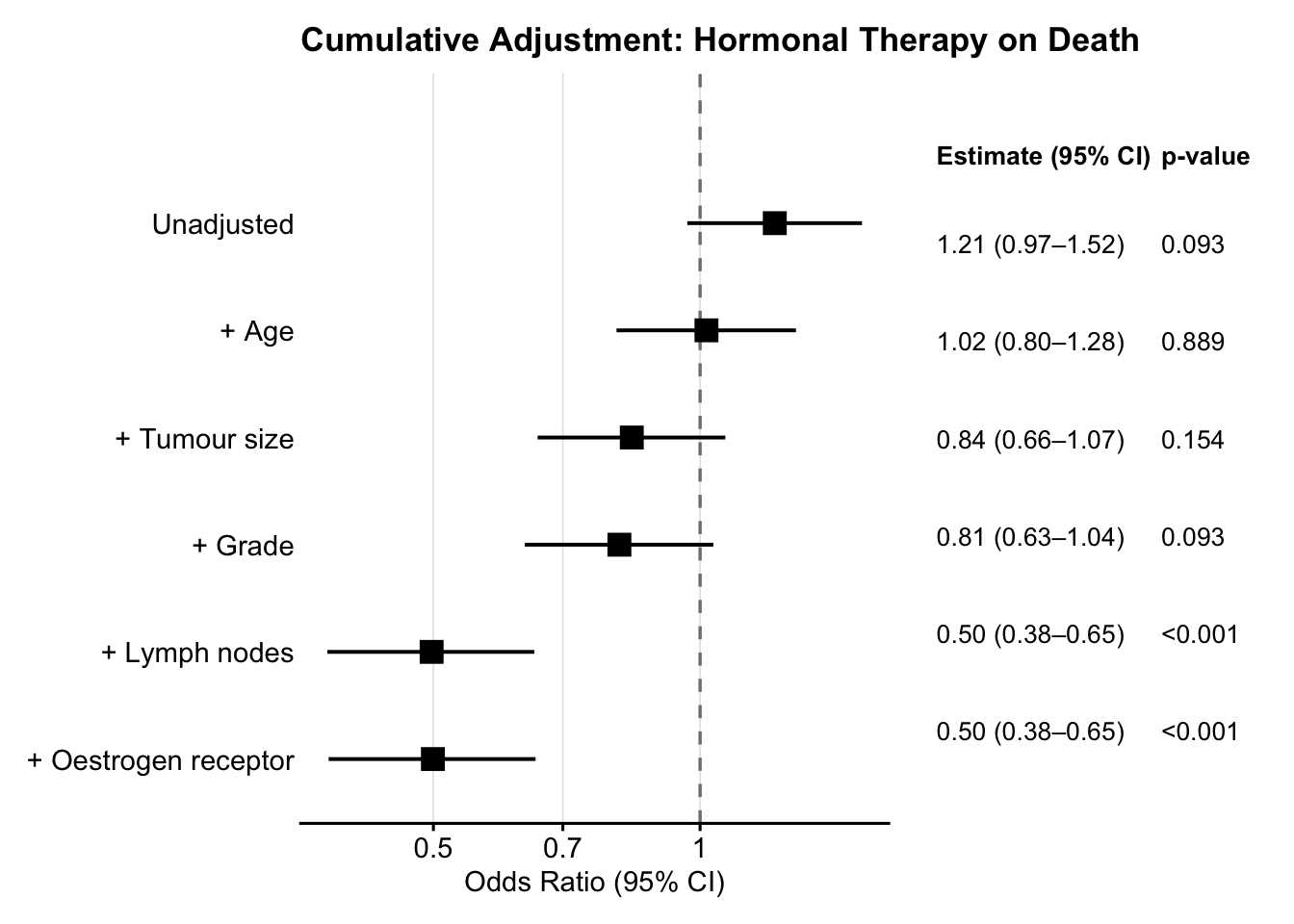
The numeric table is available for downstream use:
result_cum$formatted_table[, c("model", "formatted", "p.value")]
#> # A tibble: 6 × 3
#>   model                formatted        p.value
#>   <chr>                <chr>            <chr>
#> 1 Unadjusted           1.21 (0.97–1.52) 0.093
#> 2 + Age                1.02 (0.80–1.28) 0.889
#> 3 + Tumour size        0.84 (0.66–1.07) 0.154
#> 4 + Grade              0.81 (0.63–1.04) 0.093
#> 5 + Lymph nodes        0.50 (0.38–0.65) <0.001
#> 6 + Oestrogen receptor 0.50 (0.38–0.65) <0.001
Cox proportional hazards regression
For time-to-event outcomes supply model_type = "coxph"
along with time_var and event_var:
result_cox <- gg_adjusted_forest(
  data       = df,
  outcome    = "death",
  exposure   = "hormon",
  covariates = covariates,
  model_type = "coxph",
  time_var   = "dtime",
  event_var  = "death",
  title      = "Effect of Hormonal Therapy on Survival (Rotterdam)"
)
result_cox$plot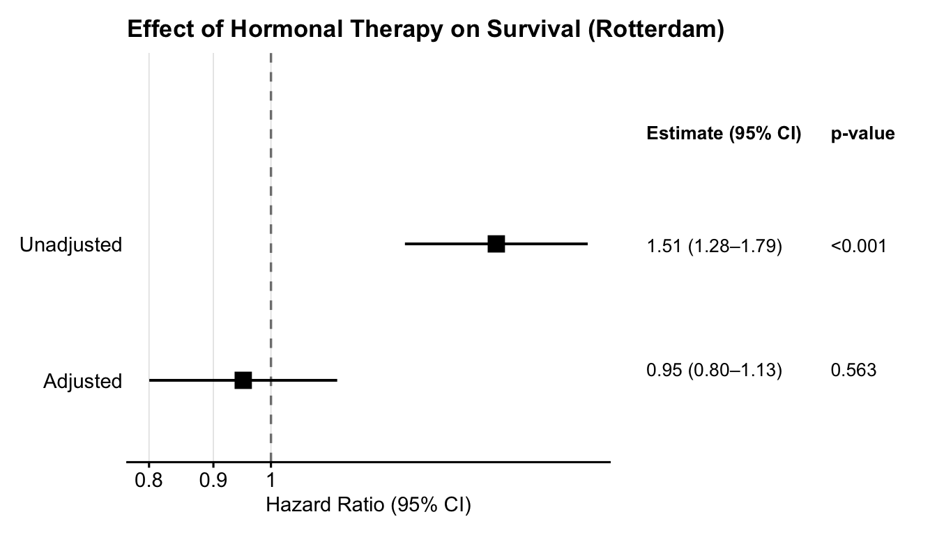
Comparing multiple outcomes side-by-side
ggadjustedforest intentionally does not provide a
built-in multi-outcome wrapper. Each outcome deserves its own carefully
specified model, and bundling them into a single function call obscures
that. Instead, fit each outcome separately and stack the plots with
patchwork, which is already a dependency of
ggadjustedforest:
library(patchwork)

p_death <- gg_adjusted_forest(
  data = df, outcome = "death", exposure = "hormon",
  covariates = covariates, model_type = "coxph",
  time_var = "dtime", event_var = "death",
  title = "Overall survival", show_table = FALSE
)$plot

p_recur <- gg_adjusted_forest(
  data = df, outcome = "recur", exposure = "hormon",
  covariates = covariates, model_type = "coxph",
  time_var = "rtime", event_var = "recur",
  title = "Recurrence-free survival", show_table = FALSE
)$plot

p_death / p_recur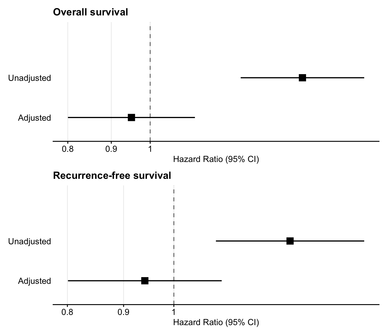
This approach gives full control over each panel — different
covariate sets, model types, or axis scales per outcome. The
/ operator stacks plots vertically; use | for
side-by-side.
Customising appearance
All the major aesthetic parameters are exposed:
gg_adjusted_forest(
  data           = df,
  outcome        = "death",
  exposure       = "hormon",
  covariates     = covariates,
  model_type     = "coxph",
  time_var       = "dtime",
  event_var      = "death",
  color          = "#2166ac",
  point_size     = 5,
  point_shape    = 18,
  vline_color    = "firebrick",
  vline_linetype = "dotted",
  title          = "Custom aesthetics"
)$plot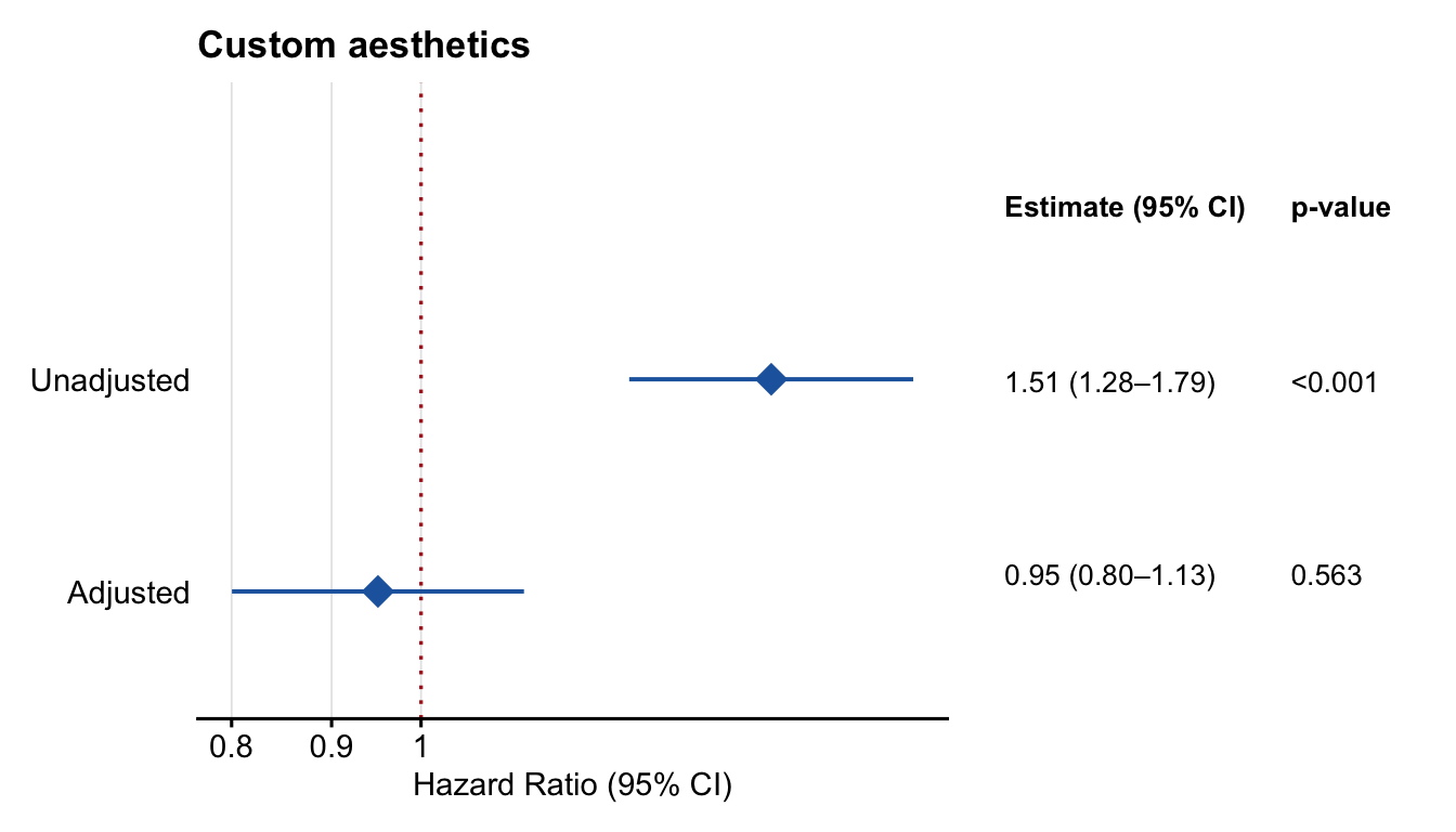
Extracting the table only
Use forest_table() when you only need the numbers:
forest_table(
  data       = df,
  outcome    = "death",
  exposure   = "hormon",
  covariates = covariates,
  model_type = "logistic"
)
#> # A tibble: 2 × 6
#>   model      estimate ci        formatted        p.value     n
#>   <chr>      <chr>    <chr>     <chr>            <chr>   <int>
#> 1 Unadjusted 1.21     0.97–1.52 1.21 (0.97–1.52) 0.093    2982
#> 2 Adjusted   0.50     0.38–0.65 0.50 (0.38–0.65) <0.001   2982
References
- Greenland S (1987). Interpretation and choice of effect measures in epidemiologic analyses. Am J Epidemiol 125(5): 761–768.
- Harrison E, Pius R (2021). R for Health Data Science. CRC Press.
- Hernán MA (2010). The hazards of hazard ratios. Epidemiology 21(1): 13–15.
- Hernán MA, Robins JM (2020). Causal Inference: What If. Chapman & Hall/CRC.
- Royston P, Altman DG (2013). External validation of a Cox prognostic model: principles and methods. BMC Med Res Methodol 13:33. (Rotterdam dataset)
- Vandenbroucke JP et al. (2007). Strengthening the Reporting of Observational Studies in Epidemiology (STROBE). PLoS Med 4(10): e297.
- Westreich D, Greenland S (2013). The table 2 fallacy: presenting and interpreting confounder and modifier coefficients. Am J Epidemiol 177(4): 292–298.
- ICH E9(R1) (2019). Statistical Principles for Clinical Trials: Addendum on Estimands and Sensitivity Analysis in Clinical Trials. ICH Harmonised Guideline.